Yield curve inversion: recession signal, but why?

The yield curve is a plot of similar fixed income securities with different maturity dates, also known as tenors. While the shape of the curve is constantly changing alongside the yields of the securities plotted, the shape of the curve tends to be upward sloping in most environments. There are many theories regarding why the curve has this upward slope, but for the purpose of this paper, we provide a brief overview of the three leading theories around yield curve shape:

1. Expectations Theory: If Investors have different expectations for the level of interest rates in the future, longer-term bonds will trade at different yield levels than shorter-term bonds. This theory states that the shape of the yield curve is a product of investors’ expectations for the path of future interest rates.  
2. Segmented Markets Theory: There tends to be different levels of investor demand for bonds of different maturities, and a varying supply of those bonds through time. This means that the interest rate for bonds of different maturities will fluctuate solely due to supply and demand, impacting the shape of the yield curve accordingly.
3. Liquidity Premium Theory: Investors require a higher interest rate for holding longer maturity bonds, because longer maturity bonds involve locking up capital for longer. This leads to an upward sloping yield curve, all else equal.

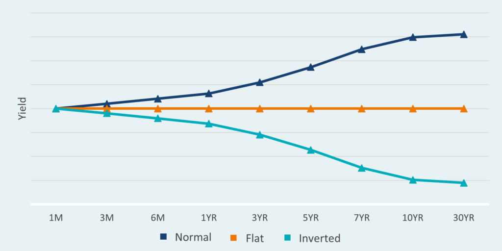
While we could write a lengthy paper reviewing yield curve theories, the emphasis of this paper is to focus on the phenomenon of an inverted yield curve, shown as the teal line in Exhibit 1 below.

Exhibit 1. Typical Yield Curve Shapes

Recession after inversion: a simpler framework

An inverted yield curve is a rare occurrence, and is characterized by higher interest rates for short-term bonds compared to longer-term bonds. As mentioned, an inverted yield curve has been one of the few consistent signals that has accurately predicted that a U.S. recession is imminent, which means that yield curve inversion tends to receive a vast amount of media coverage and attention regarding timing and signaling ability.

What has generated much less attention is why the curve inverts. Before reviewing our analysis of historical inversion periods in the next section, we lay out a simple framework to help readers better understand what drives the curve to invert.

We believe there are two key dynamics to highlight:

1. Monetary policy: The Federal Reserve’s dual mandate is to foster economic conditions that achieve stable prices and maximum sustainable employment. The Federal Reserve can influence these economic conditions by employing various measures, although their main instrument is the raising or lowering of the federal funds rate (the short-term interest rate). Increasing the rate is seen as a move to try and slow down economic activity, while lowering is meant to help incite growth. It is important to note that interest rate changes tend to have a lagged effect, which means it takes time before the impacts are fully seen in the economy.
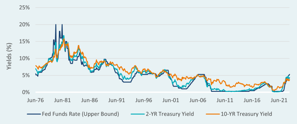
2. Short-term rates are more sensitive to changes in the federal funds rate: Short-term rates are very sensitive to the fed funds rate and track very closely. In contrast, interest rates on longer-maturity bonds, such as 10-year Treasuries, show significantly less sensitivity. This relationship can be better visualized when looking at the Exhibit 2 below, using 2 and 10-year Treasuries as our proxies for short- and long-term rates.

Exhibit 2. U.S. Treasury and FED funds rate co-movement

In short, when the Federal Reserve wishes to slow down the economy, it takes a restrictive monetary stance by increasing the policy rate, which leads short-term interest rates to rise much faster than long-term interest rates. This compresses the spread between short- and long-term rates and often leads to a yield curve inversion (short term rates being higher than long term rates). Then, this restrictive action by the Federal Reserve results in the ensuing economic slowdown that the Federal Reserve was targeting all along.

Note that not every Federal Reserve tightening cycle has resulted in an inverted yield curve. In our analysis of each period of yield curve inversion below, the yield curve inverts in periods where the Federal Reserve is combating or trying to stay ahead of inflation, compared to periods where the Federal Reserve is normalizing rates from lower more expansionary levels.

Analysis of historical inversion periods

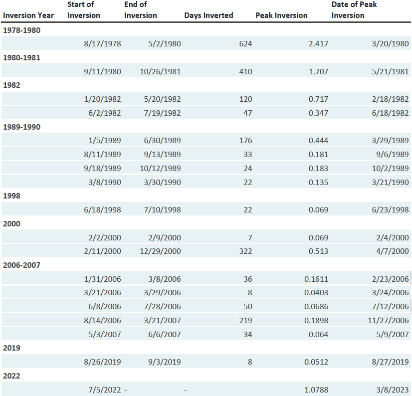
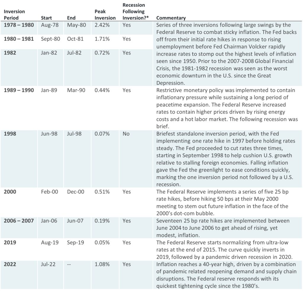
Lastly, we will look at historical periods where the yield curve has inverted. Almost every instance of yield curve inversion was followed by an economic recession six to twenty-four months after the initial inversion. We analyze macroeconomic conditions around each inversion to assist readers in better understanding what has historically driven curve inversion, while also supporting our above claim that tightening cycles to bring down or mitigate inflation have resulted in the curve inverting. Our analysis uses the spread between 2-year and 10-year treasury yields to define an inverted yield curve. Additionally, since we use daily market data dating back to 1972, we have grouped together inversion periods where market volatility saw quick movements between positive and negative spreads. The full list can be found in the appendix.

Exhibit 3. 2-10 year Treasury yield spread

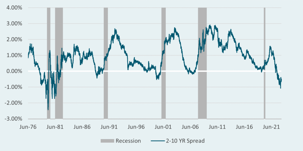
Exhibit 4. Inversion period analysis

Unique inversion periods

Two inversion periods differed from the rest: 1998 and 2019. These periods did not fit into the normal narrative of Federal Reserve tightening to slow the economy, yield curve inversion, and then subsequent recession. In this section we briefly outline these periods and illustrate why the outcomes were different.

• 1998: Strong economic growth in the early 1990’s led to a single 25 bp rate hike in March 1997 to sustain growth in a low inflation environment. The curve briefly inverted before pulling back following a series of rate cuts in order to cushion U.S. economic growth from foreign currency dynamics and slowing international growth. The backdrop of falling inflation allowed the Federal Reserve to cut rates but not cause a recession.

• 2019: In 2019, consistent rate hikes had been implemented over the prior three years. These hikes were meant to help normalize the ultra-low rate environment held by the Federal Reserve following the 2007-2008 Global Financial Crisis. The Federal Reserve had already started to cut rates in August of 2019 amid stable inflation, yet the February 2020 recession was driven by pandemic induced lockdowns (rather than the Fed’s rate hikes). This was possibly a situation where the yield curve inversion might have been an inaccurate signal, as the Federal Reserve had cushion to cut rates due to stable inflation.

Supplementary observations

In addition to our main takeaway, which presents a framework to understand the relationship between monetary policy, curve inversion, and economic slowdown, we would like to present two additional brief observations:

1. Depth of inversion seems to be dictated by magnitude of rate hikes: The depth of yield curve inversion largely seems to be a function of the size of rate hikes per Federal Reserve meeting and speed of hiking cycle. Large hikes at a quick rate suggests a larger inversion depth, as long-term rates readjust around spikes in short-term rates. Our largest inversion periods are seen in the 1980’s and 2022, which both feature quick and large hikes. On the flip side, the 17 consecutive rates hikes between 2004 to 2006 saw a peak inversion of only 0.19% despite rates increasing by 4.25%.  
2. Depth of inversion has a weak relationship with recession depth: While many readers might equate a deeper inversion with a deeper recession, this signal seems to have limited forecasting ability. This is apparent when looking at the 2007-2008 Global Financial Crisis. The Global Financial Crisis was the largest economic crisis since the Great Depression yet saw a maximum curve inversion of 0.19%.

Conclusion

In this Topic of Interest white paper, we reviewed the shape of the yield curve and leading theories on what determines yield curve shape. Next, we introduced a framework to help investors better understand why the yield curve inverts and why economic slowdown usually follows. Lastly, we supported our framework by reviewing the macroeconomic factors surrounding each yield curve inversion, while also providing two supplementary observations to assist readers trying to filter through commonly cited inversion metrics. We hope this Topic of Interest white paper allows a better understanding of why the yield curve inverts, using patterns seen in historical inversion periods to help guide decision making.

Appendix

Exhibit 5. Historical Inversion Periods

---