
Download the Topic of Interest (PDF)
Long-term asset class forecasts, or capital market assumptions, typically focus on the future performance of broad markets. However, most investors employ some combination of passive and active management in their portfolios. And active management is most often pursued with the expectation that returns will be different than that of the broad market (specifically, that “active return” will be achieved above and beyond the market return). If capital market assumptions are typically comprised of market forecasts, but investors tend to build portfolios with the expectation of market return plus active return, how might investors estimate the expected behavior of active management (active return) in their asset allocation work?¹
In this Topic of Interest we look at this question from multiple angles. First, there is not a single universal level of active return that all investors should assume. The active return that an investor might expect will depend on their specific portfolio exposures and the level of tracking error that they incur, which is driven by the investor’s individualized approach to active management. Due to this fact, we believe it is inappropriate to assume a “standard” active return in Capital Market Assumptions for use by all investors. Second, there are many ways to arrive at an active return forecast, ranging from theoretical (example: assumed information ratio) to track-record based (example: assumption that a product’s future active return will equal its historical active return), and ranging from simple to complex. We will touch on these methods and outline the merits of each. Last, we believe humility plays an important role in this process, as it is possible that aspirational active return may often exceed that which is realized. It is human tendency to have overconfidence in our abilities. Investors might consider whether conservative estimates or more aspirational estimates are appropriate for their situation.
Active return is a component of the expected return
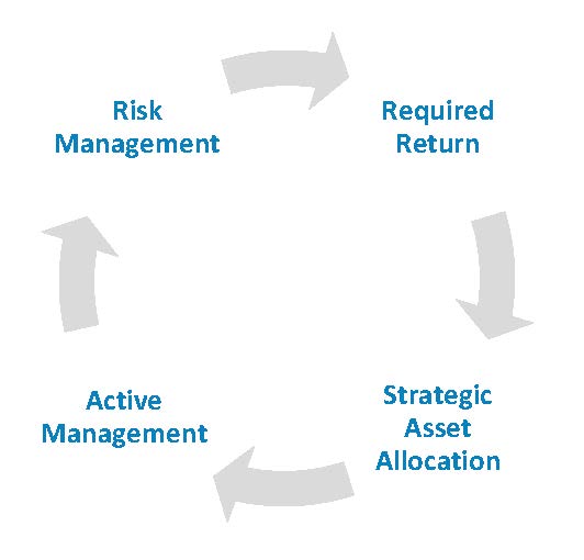
The Investment Golden Rule describes the nature of the investment problem in clear and simple terms, but without sacrificing the underlying sophistication required to construct an effective active portfolio (our Investment Golden Rule white paper can be accessed here). This framework allows investors to model future possible outcomes using a variety of approaches, and to gain an understanding of how they might succeed or fail in achieving their active management goals.
Every investor has a return objective, usually ranging from 6-8%.
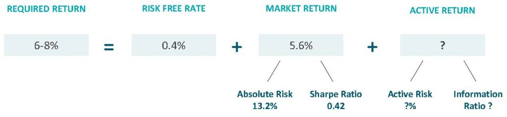
The left side of the equation defines the return goal of the portfolio—this is an input to the portfolio construction process—and setting this goal is one of the most important investment decisions. The right side of the equation details the strategy to be used to achieve that return, broken out into three sources of return: the risk-free rate, market return, and active return. The market return of the asset classes in which an investor is allocated is the major determinant of risk and return in the portfolio. Our focus in this piece is on the last component, active return, which is driven by active manager skill. The sum of these three components provides the total portfolio expected return. The job of the investor is to strike an appropriate balance across these three return sources, within an acceptable level of risk, to achieve the investor’s return objective.
The recent challenge for investors
As interest rates have fallen, and the expected market return of most asset classes has fallen due to high prices, achieving a 6-8% return will likely present greater challenges in the future.
Return expectations change over time—influenced by inflation, earnings growth, valuations and other factors. The risk-free rate is one component of a portfolio’s expected return and it has been on a secular decline since the 1980s. Figure 2 shows the magnitude by which the risk-free rate (the yield of cash) has contributed to a target return of 7%. For much of the past 100 years, the average risk-free rate was about 3%, whereas today it is nearly 0%.
3-month treasury bill rate
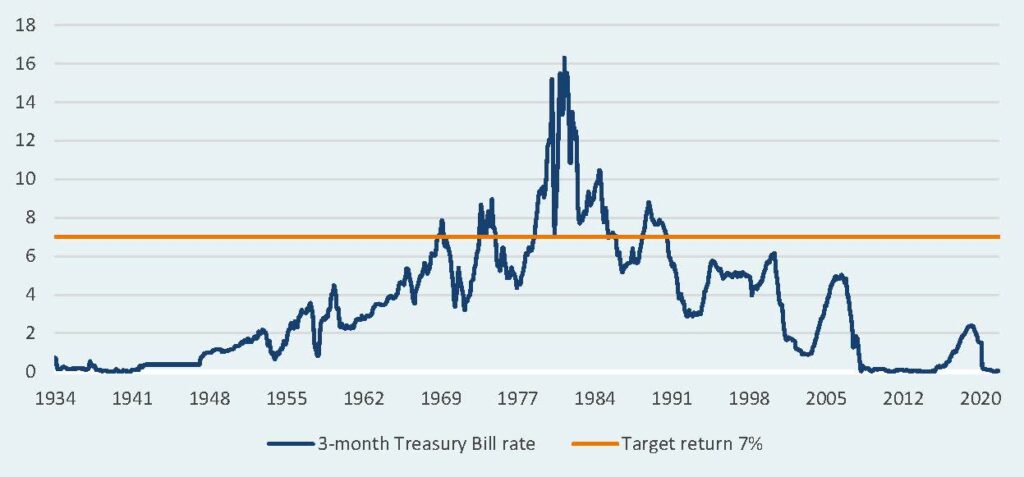
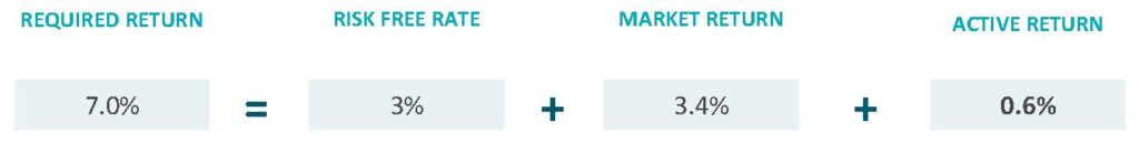
An investor could fairly easily have achieved a 7% return in the early ‘80s, however, this is no longer the case. As interest rates are nearly 0%, investors are forced to increase the return that they receive from the market and from active management in order to achieve their investment objectives. In Figure 3 we input the long-term average risk-free rate into the expected return framework. This implies that the risk-free rate and market return might have together delivered 6.4%, which is 0.6% short of the 7% return target. An active return of 0.6% could reasonably have made up this shortfall2.
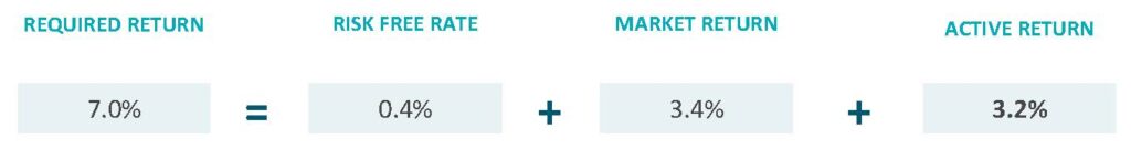
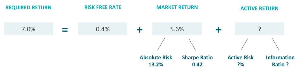
The challenge is quite different today because the expected risk-free return is 0.4%3. We highlight this dynamic in Figure 4, which implies an investor today would need to achieve an active return of 3.2% to meet an expected return of 7%. This portfolio would require a significantly different active structure relative to the portfolio that was only targeting 0.6% of active return. In reality, an investor would likely choose to reexamine both their portfolio market return and active return goals to make up for a 3.2% shortfall.
The exercise of identifying each interrelated expected return component provides insight into the investment program. This creates a roadmap for how returns will be achieved and can help investors make more informed decisions. This framework allows investors to easily identify how much active return they need to target to achieve return objectives. Once an investor defines how much active return they need to target, then they can develop a plan to achieve that goal.
The pursuit of active return may require a greater focus on:
- Active management: Changing the active/passive structure in a portfolio involves identifying asset classes that are less efficient and therefore might provide greater opportunity for active managers to add value. Verus produces an annual active management environment piece that reviews the efficiency of each asset class, which can be accessed here.
- Taking on additional risk: An investor may decide which areas of the portfolio are likely to provide the best opportunity for active return and will likely decide to take on greater active risk in those areas. Active risk is therefore allocated across the portfolio by allowing managers to pursue this type of risk in asset classes with the greatest chance of success (we discussed this in our white paper Managing and Budgeting Active Risk, which can be accessed here).
- Increased portfolio complexity: This may come in the form of adding portable alpha strategies or allocating to alternative investment managers.
- Higher allocations to illiquid assets: Increasing allocations to private equity, private credit, infrastructure, real estate, etc. These markets tend to be less efficient and provide opportunities to increase active return potential. We discuss this dynamic in our strategic liquidity white paper.
The decision for how to pursue active return is dependent on the risk tolerance and governance policies of each investor. The Investment Golden Rule makes these payoff choices clearer, makes them more understandable and less emotive, and makes them available for all the people around the table, no matter what their experience level.
Active return is informed by approach
The active return that an investor might expect will depend on their approach to active management, their tracking error budget, and their specific portfolio exposures. Just as an investor’s expected portfolio return is based on that investor’s approach to asset allocation, each investor’s expected active return will be based on that investor’s approach to active management.
First, an investor’s approach to active management will affect the expectations for active return. For example, for some investors the value of active management is risk reduction relative to the benchmark, rather than higher returns. Certain active managers possess skill to deliver benchmark-like returns but at lower levels of risk than the benchmark. In this case, an active return forecast may in fact be 0%, as the expected value from active management is from the risk side of the equation. Low volatility equity strategies may serve as an example here4.
Second, tracking error is necessary but not sufficient for generating active return. Active managers will need to take on tracking error in order to deliver active return, but tracking error does not guarantee that added return. In simpler terms, active managers need to take positions different than the benchmark (tracking error) to add value, but those positions of course also need to be profitable ones (skill). Active return is not a commodity that is simply manufactured from tracking error, but the size of an investor’s tracking error budget for each asset class is an important variable for estimating this return.
Last, the specific exposures in a portfolio should inform active return estimates. We say this because certain asset classes may provide a better hunting ground for active return than others. For example, the U.S. large cap public equity market is generally believed to be a fairly efficient market, relatively speaking, while the emerging market equity segment is believed to be less efficient. The historical success rate of active management differs from asset class to asset class, and history may serve as a guide for forward-looking return estimates.
This suggests that, rather than recommending a single assumed active return number for an asset class for all clients, an assumed return figure should be calculated for each client for each asset class, based on the implementation approach proposed.
There are many ways to forecast active return
Many approaches have been developed over the years which might be used to forecast active return. These approaches range from highly complex and time intensive to very simple and intuitive. As we believe is often the case, simple is not necessarily inferior and may be preferable, especially in a portfolio-wide context when an investor is developing active return forecasts for multiple asset classes. In the table below we outline examples of various methods to estimate active return.
Examples of active return forecasting methodology
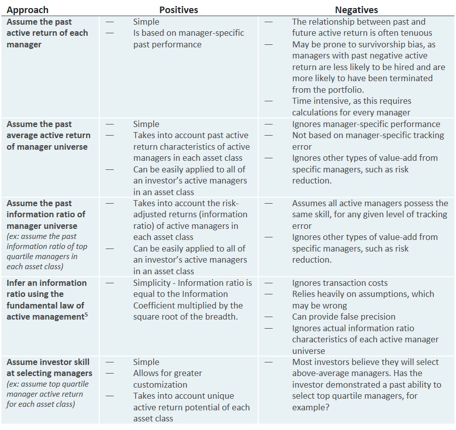
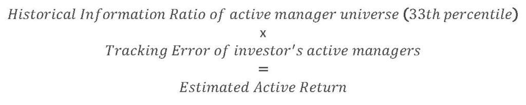
Investors will, and do, employ many different methods for tackling active return estimation. The preferred method will likely be decided by the investor’s willingness and capacity to devote major resources to this exercise, and their confidence that more resources will indeed improve the estimate (as mentioned, we do not believe that complexity is always additive). For most investors, most of the time, we believe that it is reasonable to calculate the historical information ratio for each individual asset class (each active manager universe), and to use this universe average, along with the tracking error of the investor’s actual active managers, to arrive at expected active return. Historical universe information ratio might be defined as the average manager information ratio of the universe, if an investor chooses to be conservative in their active return estimate (i.e. assume that they will achieve an “average” information ratio). Or it could involve the top quartile universe information ratio (25th percentile), if an investor is confident in their ability to select top quartile managers. If the latter, the formula used to estimate active return for a single asset class is as follows:
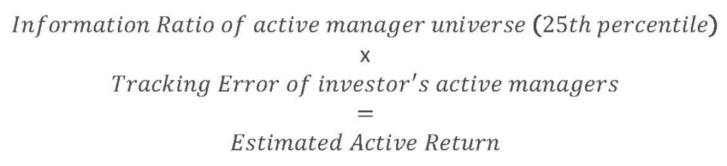
This formula provides the following benefits: 1) it is simple and fairly quick to calculate, 2) it is realistic with regard to the actual information ratios achieved broadly by active managers in each asset class, 3) it integrates the actual tracking error of an investor’s underlying active managers.
A worked example: tying all of these concepts together
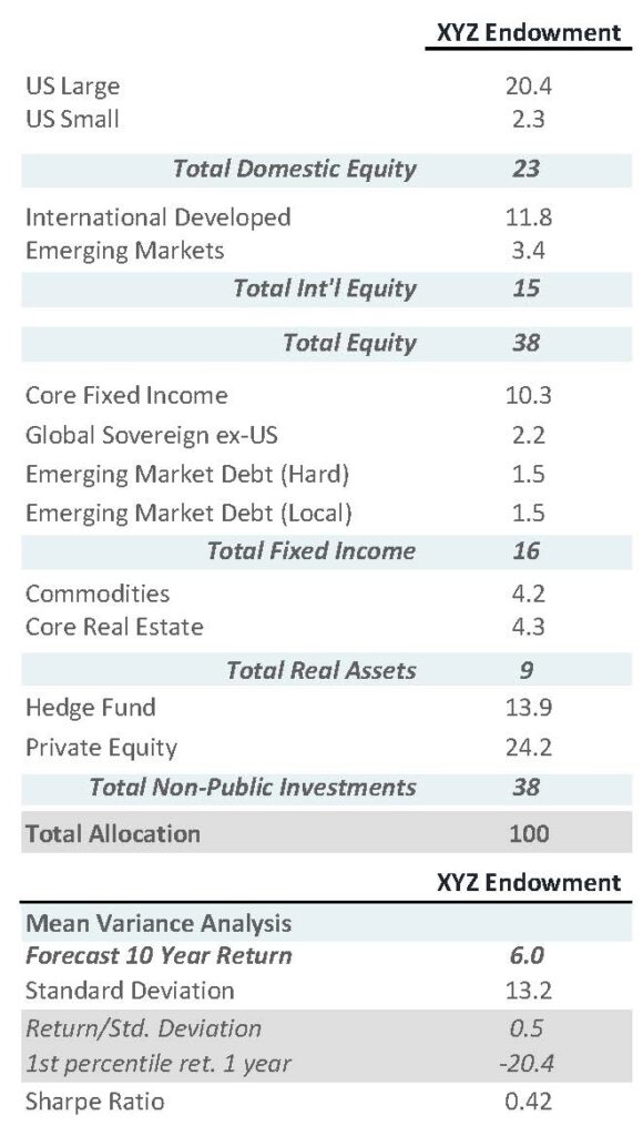
Now let’s briefly work through how this methodology might be followed in practice. In our example below, investor XYZ Endowment is putting together an asset allocation study as a part of their annual process. XYZ Endowment targets a 7% annual return and traditionally excludes any active return assumptions from their asset allocation discussions, but has decided this year to integrate active return into their process. As a first step, XYZ Endowment works with their consultant to calculate their portfolio expected return as per their usual process (excluding active return). This investor calculates the long-term portfolio expectations using their consultant’s Capital Market Assumptions, shown below.
XYZ Endowment asset allocation & expected return (excluding active return)
Next, XYZ Endowment follows the Investment Golden Rule framework, and inputs the assumptions above into this formula.
Investment Golden Rule framework
The endowment now must decide how to best forecast the active return of their portfolio, in effect filling out the third component of the Investment Golden Rule formula. The investment committee begins by reviewing the merits of a variety of approaches to forecasting active return.
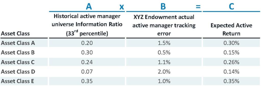
The committee comes to the agreement that a reasonable and conservative approach would be to assume their active managers possess the skill to perform among the top one third of managers in each respective universe. The committee also agrees that historical information ratios of individual active management universes will likely provide a reasonable guide as to future information ratios6. Restated in mathematical terms, XYZ Endowment has decided to forecast active return using the formula below, for each standalone asset class.
Next, the committee works with their consultant to calculate active return forecasts for each asset class, as illustrated below.
Finally, XYZ Endowment integrates these active return forecasts into the original asset allocation study to arrive at an updated total portfolio expected return. The updated total portfolio expected return is displayed below in the Investment Golden Rule framework.
Investment Golden Rule framework (updated with Active Return)
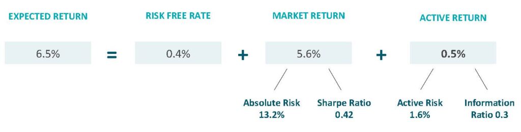
The updated Investment Golden Rule formula now includes an active return component, and provides the endowment with a more holistic picture of likely future portfolio performance.
It is possible that an upcoming discussion at XYZ Endowment will revolve around the fact that the portfolio expected return of 6.5% is 0.5% short of their 7% target. The active return forecasting framework presented in this white paper may also assist in that discussion. As demonstrated in the formula above, XYZ Endowment could choose to increase the portfolio expected return by adjusting asset allocation (i.e. adjusting “market return”), or could choose to pursue greater added value from active management (i.e. adjusting “active return”), or might pursue some combination of both. If greater active return plays a role in reaching for higher portfolio returns, the Investment Golden Rule demonstrates that greater active return might be achieved in a variety of ways:
- The pursuit of higher tracking error across the portfolio
- Greater focus on active management within less efficient asset classes (example: those with higher average active manager information ratios)
- Allocations to highly skilled active managers
Active return is of course not an unlimited resource. Each investor will need to evaluate the level of value added that is reasonable to expect, given their allocations and approach to active management.
The importance of humility
“Welcome to Lake Wobegon, where all the women are strong, the men are good looking, and all the children are above average.” -Garrison Keillor
“Lake Wobegon”, a fictional town as imagined by Garrison Keillor, is an idyllic place which might resemble many small Midwest towns. The psychological human tendency to overestimate one’s own capabilities is often referred to as the “Lake Wobegon effect”, in reference to Keillor’s fictional town. Ola Svenson discovered that 80% of U.S. survey respondents rated themselves as being in the top 30% most skilled automobile drivers7. Asking college students about their popularity, Zuckerman and Jost demonstrated that most students believe themselves to be “more popular than average”8. This behavioral effect has been demonstrated in countless other national studies, applying to college students, educational professionals, business executives, and, yes, even investors. To put it bluntly, it is human nature to believe that we are all above-average, when in fact many of us (half, to be exact) are not. It is a mathematical certainty that this also applies to the achievement of active return—while most investors believe that the active managers they have hired will deliver top quartile (or even top decile) performance, this is not possible for everyone. In fact, the true “average” active return from active management is 0%, or indeed often negative after fees.
“There is a constraint on the returns to active investing that we call equilibrium accounting. In short, suppose that when returns are measured before costs (fees and other expenses), passive investors get passive returns, that is, they have zero α (abnormal expected return) relative to passive benchmarks. This means active investment must also be a zero sum game—aggregate α is zero before costs. Thus, if some active investors have positive α before costs, it is dollar for dollar at the expense of other active investors. After costs, that is, in terms of net returns to investors, active investment must be a negative sum game. (Sharpe (1991) calls this the arithmetic of active management.)”9
Eugene Fama & Kenneth French
And this creates a bit of a conundrum, if most (or all) investors assume they will achieve positive active return in the future when in fact half (or more) of those investors will achieve negative active return. We believe that the degree to which an investor should lean more aspirational or conservative in their level of active return assumptions is a somewhat personal choice based on individual circumstances. Humility should play a role in this decision in order to set realistic and achievable expectations.
Conclusion
Capital market assumptions are typically comprised of “market return” forecasts, but investors tend to build portfolios with the expectation of market return plus “active return”. In this Topic of Interest we examined how investors might integrate the expected behavior of active management (“active return”) into their asset allocation work. First, we outlined the reasons why there is not one universal level of active return that all investors are entitled to. The active return that an investor might expect will depend on their specific portfolio exposures and the level of tracking error that they incur, which is driven by the investor’s individualized approach to active management. Due to this fact, we believe it is inappropriate to integrate a “standard” active return number into Capital Market Assumptions for use with all clients. Second, we discussed the many ways that an investor might arrive at an active return forecast, ranging from theoretical (ex: assumed information ratio) to track-record based (ex: assumption that a product’s future active return will equal its historical active return). We walked through these practices and discussed the merits of each, as well as our preferred approach. Last, we touched on the role which humility might play throughout this process, as it is possible that realized active return may fall short of aspirational active return. Investors might consider whether more conservative estimates or more aspirational estimates are appropriate for their situation. For additional details regarding our thinking on these topics, please reach out to your Verus consultant.
1 Investors sometimes refer to outperformance over the market return as “alpha”. However, “alpha” is the risk-adjusted outperformance over market return. We use the technically correct term here, “active return”, also known as “excess return”.
2 Of course, an investor may instead decide to increase their market exposure (beta) to make up for this 0.6% return shortfall, or may pursue a combination of beta and alpha.
3 Using Verus’ Capital Market Assumptions. We assume the same beta return in this example.
4 The Low Volatility Equity effect is grounded in the historical observation that less volatile stocks tend to product superior risk-adjusted performance, or even superior absolute performance. Verus has conducted research on this effect and has found that the least volatile active management strategies tend to produce superior risk-adjusted returns across most time periods and most major asset classes examined.
5 Kahn, Ronald, “Seven Quantitative insights into Active management Part 3: The Fundamental Law of Active Management. 1997.
6 “Information Ratio” is defined an active manager’s average performance relative to that manager’s benchmark performance, divided by the volatility of the return difference between active manager performance and benchmark performance. In simpler terms, Information Ratio is the risk-adjusted active performance of a manager.
7 Svenson, O. (1981). Are we all less risky and more skillful than our fellow drivers? Acta Psychologica, 47, 143-48.
8 Zuckerman, E. W., & Jost, J. T. (2001). What Makes You Think You’re So Popular? Self Evaluation Maintenance and the Subjective Side of the “Friendship Paradox”. Social Psychology Quarterly, 64(3), 207-223.
9 Fama & French (2010). Luck versus Skill in the Cross-Section of Mutual Fund Returns. Journal of Finance Vol LXV No. 5 p. 1